Playing Pokemon Grow with Differentiable Cellular Automata
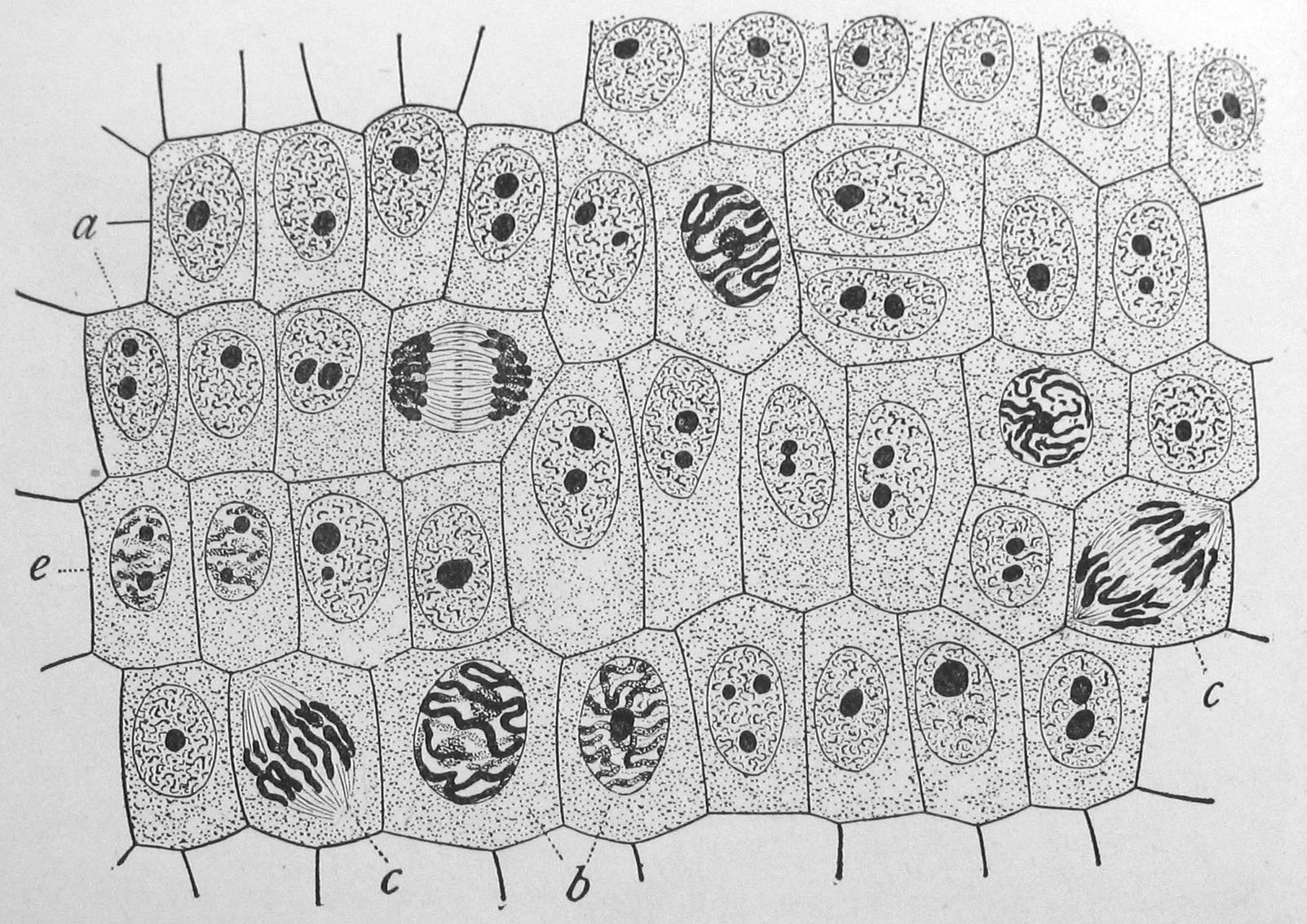
From Wilson, Edmund B. The cell in Development and Inheritance (2nd ed.) 1900. Public Domain from Wikipedia.
#/media/File:Wilson1900Fig2.jpg)
Look back to the 1980s and you’ll find that, alongside a vibrant wave of connectionism that laid the foundations for the deep learning renaissance of the 2010s, there was an enthusiastic community of researchers working on cellular automata (CA). They were mentioned in Richard Feynman’s keynote “Simulating Physics with Computers” (Feynman 1981) as a candidate computational paradigm for physics, and in particular Feynman liked the locality properties of CA. In general each cell only receives information from a local neighborhood, and this characteristic is considered attractive for scaling purposes.
Communication represents one of the largest components of the energy budget for modern computation (Miller 2017), and a practical consequence of long interconnects in computers is that, for deep learning models, memory access can dominate total energy consumption. Communication is such an energy sink in computation that compressing deep learning models to fit into on-chip SRAM can decrease total energy costs by about 120 times, compared to the same model prior to compression that needs to read from off-chip DRAM memory (Han et al. 2016). That’s one reason why systolic arrays make attractive building blocks for machine learning accelerators like Google’s line of TPUs (Kung 1982 pdf). Systolic arrays, like CA systems, are made up of many relatively self-contained compute units each with their own memory and simple processor. Connections in systolic arrays are local, and just like the abstraction of CA, information flows through many cells, undergoing computation along the way.
There are marked mathematical similarities between CA and neural networks. In fact, work from William Gilpin showed that generalized cellular automata can be readily represented in a special configuration of convolutional neural network (Gilpin 2019). That’s reflected in practice in how modern CA researchers use deep learning libraries like TensorFlow or PyTorch for both computational speedups and automatic differentiation. Despite the shared formulation and convenience of implementing CA with neural network primitives, it’s supposedly somehow still difficult for neural networks to learn the most famous set of CA rules, John H. Conway’s Game of Life (Springer and Kenyon 2020).
Like other AI-adjacent topics, the roots of cellular automata go back much further in time than contemporary research trends, with John Von Neumann introducing his 29-state rules in 1966 (Von Neumann and Burks 1966) and Conway’s famous Game of Life described in Scientific American by Martin Gardner in 1970 (Gardner 1970 pdf). We’ll leave the historical treatment for another time, but it’s worth being aware of the rich legacy of CA work and discoveries by hobbyists and professional researchers alike.
In this essay we are concerned with the synergistic combination of CA and differentiable programming. Unlike classical CA, these systems are parameterized with continuous-valued parameters. Recent work has demonstrated continuous-valued, differentiable CA as a model for development and regeneration loosely based on biological embryogenesis (Mordvintsev et al. 2020) and “self-classifying” MNIST digits (Randazzo et al. 2020)—an approach to image classification that naturally lends itself to semantic segmentation (Sandler et al. 2020). That pair of papers were published in the same month, with Sandler et al.’s segmentation paper coming out a few weeks before Randazzo et al.’s similar MNIST classification demonstration. I’ll argue here that differentiable CA (also referred to as neural CA, or NCA, in the literature) represent a promising, albeit nascent, research direction that is currently under-appreciated.
CA have the following, non-comprehensive, desirable characteristics that make them attractive as a potential alternative to conventional deep learning models:
-
They hold some promise as an avenue for a parsimonious learning machine. A CA ruleset optimized for a given task may offer simplification over conventional deep networks, but with the potential for training meta-learning CA we may additionally find recipes for compact and generalizable sets of learning rules that can operate on grids or graphs. Simpler models are also preferable for having lower running costs.
-
They are ideally suited for efficient computation on present and upcoming machine learning hardware accelerators, and conveniently suited for implementation with existing deep learning libraries. Also, they may be well-suited for asynchronous computation, which heels closer to what we might intuit about the workings of biological nervous systems.
-
They offer computational flexibility in that computation costs can be balanced against accuracy or uncertainty thresholds by dynamically adjusting the number of CA steps.
In short I think that CA are a reasonable area of research to pursue with strong potential for both applied utility and basic AI research. As a “path less traveled,” even if CA are ultimately found to be less effective or less efficient in most use case, the endeavor will still offer lessons on the nature of learning at the very least. If CA offer nothing more than equivalent performance to conventional deep learning but in simpler form, it’s a worthwhile pursuit for mitigating issues of environmental impact and societal inequality that can be exacerbated by modern machine learning practice. Consider that Emma Strubell and colleagues estimated the energy requirements of training a large NLP model with hyperparameter and architecture search has a carbon impact of about 5 times that of an average car over its entire lifetime (Strubell et al. 2019) and that estimates for monetary costs (at retail price) of compute used for headline deep learning projects typically fall into the range of tens of millions in USD. The high cost of deep learning is unsatisfying in its own right, as we know that general intelligence can be enacted with an energy flux of some tens of Watts, as we see in human brains.
For the work described here, I used the Pokemon Images Dataset from kvpratama on Kaggle.
Training Differentiable Cellular Automata
In this essay I’ll describe training differentiable CA for constructing images of Pokemon from noisy, heavily truncated initial conditions. The training regimen is similar to that described by Mordvintsev et al., with a CA implementation in PyTorch is structurally similar to that of Gilpin. CA rules are represented by a set of two convolutional layers with 1x1 kernels, and each cell in the CA state grid is defined by a 16-element vector, with the first 4 elements being interpreted as RGB intensity and transparency. I used alive masking and stochastic cell updates as in Mordvintsev et al.
Training perturbations
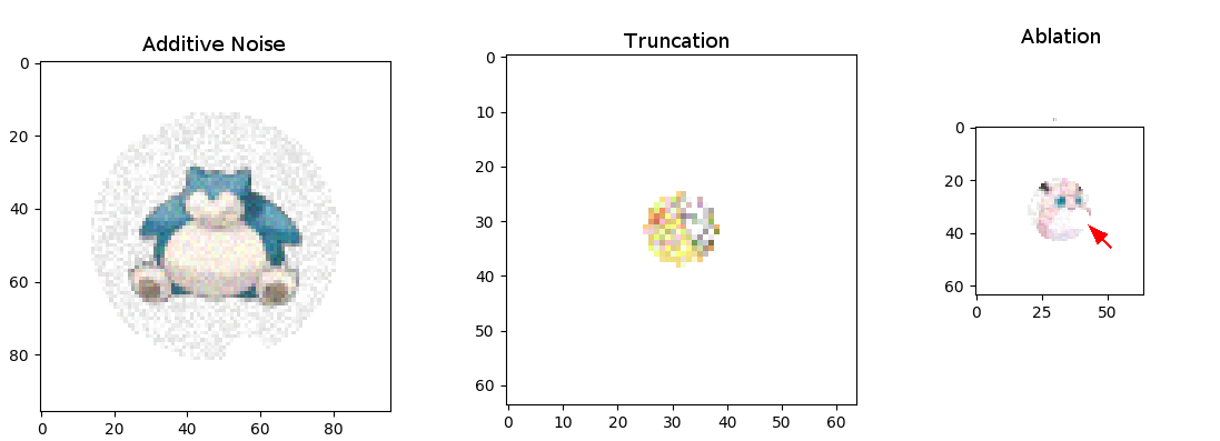
During training input images are subjected to 3 types of perturbation: additive noise, truncating the image according to a maximum radius about the image center, and ablating circles of pixels around random coordinates. For the work described here, perturbations are applied only at the first time step, but we could conceivably train more resilient CA by applying perturbations at random intervals.
Departing slightly from the training described in (Mordvintsev et al. 2020), I use an incremental difficulty that is modulated in keeping with improved CA performance. This is accomplished by increasing the severity of input image perturbations when the model passes a performance threshold, as well as increasing the number of steps. In the beginning, the input image is essentially a slightly noisy version of the target image, and by the end it amounts to a heavily cropped version with substantial noise and missing pixels. You could consider this as an approximation of training from the last few steps at the start, and gradually moving the starting point backward in terms of the number of steps to reach a solution. In my experience so far this helps prevent the CA model from getting stuck in a local minimum (e.g. by zeroing out all the cells) from which it doesn’t generate a useful error signal sufficient to escape.
I trained 3 separate models with 3 separate Pokemon, one for each perturbation. The result is 3 models each specialized to a given task and monster: persistence (Charizard), growth (Pikachu), and healing (Jigglypuff). If you are disappointed that I left out your favorite Pokemon, I am sorry (sort of), but you can always have a go at training based on the code in the project repo.
CA Model Formulation
As alluded to earlier, I implemented cellular automata rules as a series of two convolutional layers. The first is split into convolution with Sobel edge filters and a Moore neighborhood kernel, and generates the perception that feeds into the CA ruleset. The second layer applies the CA ruleset with several channels of 1x1 convolutional kernels. That formulation is in turn an implementation of applying the same dense multilayer perceptron model to each cell. We’ll look at the CA function first.
def update(perception, weights_0, weights_1, bias_0, bias_1):
    """
	returns a state_grid based on a computed neighborhood grid
	i.e. the perception tensor
	weights are NxCx1x1, i.e. convoluation uses one by one kernels
    """

    groups_0 = 1
    use_bias = 1

    if use_bias:
        x = F.conv2d(perception, weights_0, padding=0, groups=groups_0, \
		bias=bias_0)
    else:
        x = F.conv2d(perception, weights_0, padding=0, groups=groups_0)

    x = torch.atan(x)

    groups_1 =  1

    if use_bias:
        x = F.conv2d(x, weights_1, padding=0, groups=groups_1, \
		bias=bias_1)
    else:
        x = F.conv2d(x, weights_1, padding=0, groups=groups_1)

    x = torch.sigmoid(x)

    return x
The input (variable perception in the function update) needs to have some sort of local connections to surrounding cells, otherwise there’s no way for information to travel through the state grid and cell states will only ever depend on their own history. We follow (Mordintsev et al. 2020) in using Sobel filters to calculate an edge-detection neighborhood, as well as incorporating a traditional Moore neighborhood and concatenating the previous time step’s state as part of the perception input.
def get_perception(state_grid, device="cpu"):

    my_dim = state_grid.shape[1]
    moore = torch.tensor(np.array([[[[1, 1, 1], [1, 0, 1], [1, 1, 1]]]]),\
            dtype=torch.float64)
    sobel_y = torch.tensor(np.array([[[[-1, 0, 1], [-2, 0, 2], [-1, 0, 1]]]]),\
            dtype=torch.float64)
    sobel_x = torch.tensor(np.array([[[[-1, 2, -1], [0, 0, 0], [1, 2, 1]]]]), \
            dtype=torch.float64)


    moore /= torch.sum(moore)

    sobel_x = sobel_x * torch.ones((state_grid.shape[1], 1, 3,3))
    sobel_y = sobel_y * torch.ones((state_grid.shape[1], 1, 3,3))
    sobel_x = sobel_x.to(device)
    sobel_y = sobel_y.to(device)

    moore = moore * torch.ones((state_grid.shape[1], 1, 3,3))
    moore = moore.to(device)

    grad_x = F.conv2d(state_grid, sobel_x, padding=1, groups=my_dim)
    grad_y = F.conv2d(state_grid, sobel_y, padding=1, groups=my_dim)

    moore_neighborhood = F.conv2d(state_grid, moore, padding=1, groups=my_dim)

    perception = torch.cat([state_grid, moore_neighborhood, grad_x + grad_y], \
		axis=1)

    return perception
Like the work by Levin and colleagues published on Distill, I used stochastic updates to mimic asyncrhonity. In this scheme, some percentage (I used 20%) of the state grid are left unchanged at each update step. The motivation behind stochastic updates is to encourage models to learn robust rules that would perform well on low-energy asynchronous hardware, and I strongly suspect that stochastic updates can act as a powerful regularization tool akin to dropout.
In between each update, cells are zeroed out if their alpha value, represented as the fourth element in each cell’s state vector, falls below 0.1. Those cells are considered “dead” and this is intended to clean up transparent pixels at each step.
def stochastic_update(state_grid, perception, weights_0, weights_1, bias_0, bias_1, rate=0.5):

    # call update function, but randomly zero out some cell states
    updated_grid = update(perception, weights_0, weights_1, bias_0, bias_1)

    # can I just use dropout here?
    mask = torch.rand_like(updated_grid) < rate
    mask = mask.double()
    state_grid = mask * updated_grid + (1 - mask) * state_grid

    return state_grid

def alive_masking(state_grid, threshold = 0.1):
    # in case there is no alpha channel
    # this should only take place when loading images from disk
    if state_grid.shape[1] == 3 and state_grid.shape[0] == 1:
        temp = torch.ones_like(state_grid[0,0,:,:])

        temp[torch.mean(state_grid[0], dim=0) > 0.99] *= 0.0
        state_grid = torch.cat([state_grid, temp.unsqueeze(0).unsqueeze(0)], dim=1)

    # alpha value must be greater than 0.1 to count as alive
    alive_mask = state_grid[:,3:4,:,:] > threshold
    alive_mask = alive_mask.double()
    state_grid *= alive_mask


    return state_grid
That’s it for the essential functionality of a differentiable cellular automata model. To peruse the details of training and how data are prepared, check out this project’s Github repository.
After training for a while on a PIkachu sprite, a CA model can learn to reproduce a reasonable facsimile of the creature’s image based on highly constrained starting conditions.
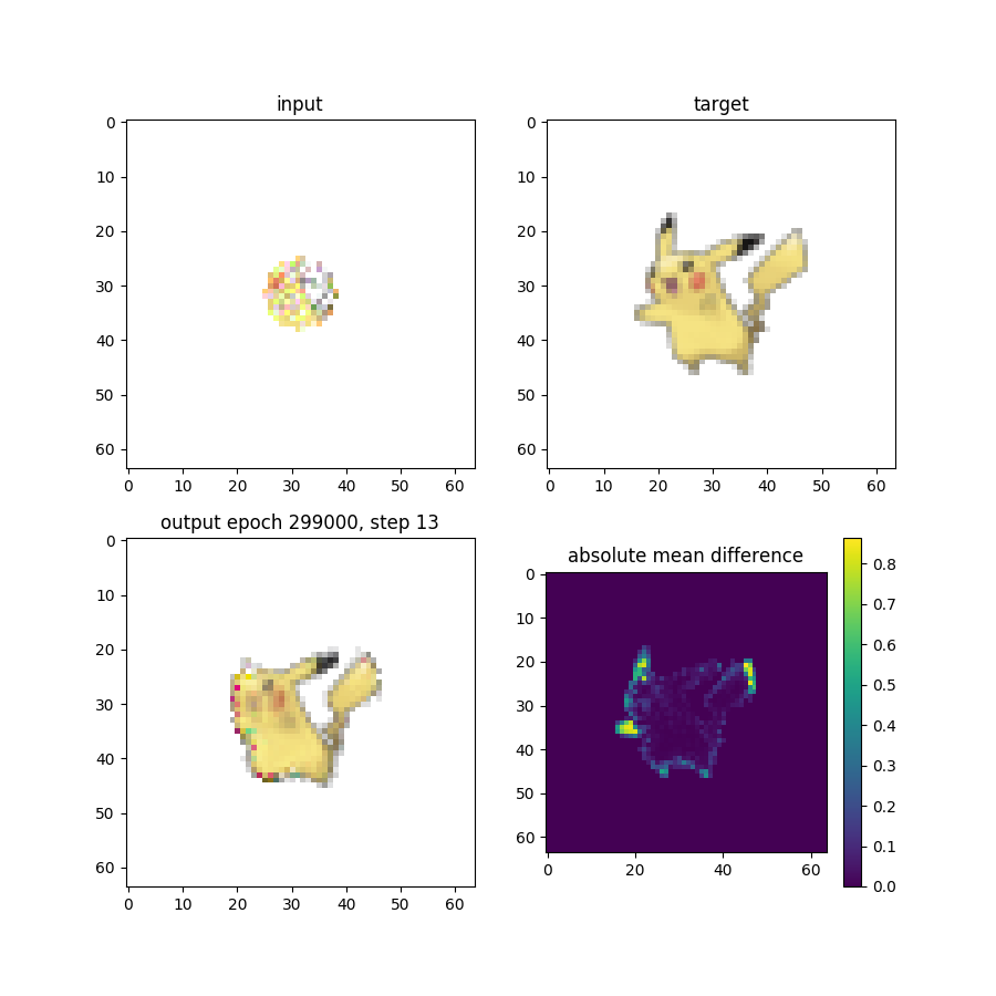
Reconstructing Pikachu necessitates a model that learns how to grow ears, paws, and a tail, all of which are cut off by the truncation perturbation described earlier. It’s frankly pretty cool to see it working, but with the capacity for growth comes the capacity for something much more sinister.
Given that we’re working with Pikachu here, it should come as no surprise that things take a dark turn eventually. Like the willfully naive paperclip maximizer thought experiment, some training conditions will result in a model that won’t be satisfied until it turns its entire universe into Pikachu. This shouldn’t be too surprising, as a basic training configuration only considers a few time steps at the end when formulating the loss function. Expecting state grids from before or after the steps used for the loss function to yield good results is like looking for realistic images in the early hidden layers of a GAN generator, or continuing with arbitrary convolutional layers after the output layer and expecting those to look good as well.
I’ve tried a few methods for stabilizing training in growth models, mainly by adding a second sampling protocol for calculating the loss function. Currently this tends to make training unstable and leads to a dead CA universe where all cells eventually fail to meet the requirement to pass information through the alive masking step. While technically a dead universe accomplishes the intended goal of stability, it’s hardly desirable. For now we are stuck with a somewhat malignant Pikachu growth model. I am only allowed to come up with one joke a year, and while technically it is now 2021 my humor accountant says I can designate the following figure caption to the 2020 joke year, leaving at least one more gem of comedy gold for you to look forward to from yours truly in 2021.

In the Pikagoo scenario, out-of-control self-replicating Pikachu cells consume all mass on Earth while building more of themselves. Ranked in the top 10 doomsdays in a survey of "expert" (that's me, I made it up). Here shown running at 3x speed.
And here’s an example of a Pikachu CA rule “infecting” an image of a Snorlax. The Pikachu CA takes hold pretty quickly, so I froze the starting image for the first 8 frames.

Watching the persistence model for Charizard is decidedly less exciting.

Perhaps the most compelling example is Jigglypuff, for which I trained a set of CA rules for damage recovery. Regrowth/healing CA rules are one of the interesting from a fundamental research perspective (especially if combined with an effective stable growth strategy). It’s not too much of an intellectual leap to go from repairing an image to repairing/updating an intelligent agent policy in a changing environment.
The Pokemon CA models described in this essay are each trained on a single sample image, so the concept of generalization doesn’t really apply (yet). Training differentiable CA is tricky, I’d say somewhat more difficult than building and training your own GAN from scratch, but it looks awesome when it works out. Over the next year or so I expect to see development of differentiable CA for many of the toy and demo problems on images readily solvable by convolutional neural networks. Image processing will probably provide the first “low-hanging fruit,” (as we’ve already seen with CA for classification and segmentation), but I predict we’ll also see CA as a powerful tool for meta-learning in keeping with noted similarites to developmental biology. I’ll be working on some of these problems myself, so stay tuned if that sounds like something you’d be interested in.
Anyway, here’s Wigglytuff subjected to the Jigglypuff CA (shown at 8x speed) in a poignant visual metaphor of the saying “You can’t go home again”:
