Improving the Scoring Function for Protein-Ligand Docking with Evolutionary Reinforcement Learning
Proteins, an Ancient Type of Micro-Robot
I don’t know about you, but I have a rich inner life of warm, wet, and squishy nanomachines slamming into each other at excessive speeds. Every once in a while, one of these relatively gargantuan machines will slam into a much smaller object and the two will stick together for a while. The interaction between the two may totally change the activity of the larger nanomachine or even physically change the smaller partner, and when things go wrong in how they interact bad outcomes may result. This rich inner life is sometimes invaded by bad information, co-opting my machinery to build other things that don’t help me out at all.
I’m talking, of course, about proteins and their binding partners, known as ligands. Of all the types of biological macromolecules (also including lipids, polysaccharides, and nucleic acid polymers), proteins are some of the more obvious pieces of the biological puzzle in terms of their phenotypic functionality. As a result, understanding how small molecules perturb protein activity is a big part of understanding health and disease, and a key to modifying normal and pathological behavior. Ligands can be many things: peptides, nucleotides, or small molecules. Today we will focus on the latter category of small molecules, as these are often good candidates for effective drugs.
Take the molecular structure shown below. You’re likely familiar with the substance if not the exact structure and interacting protein.
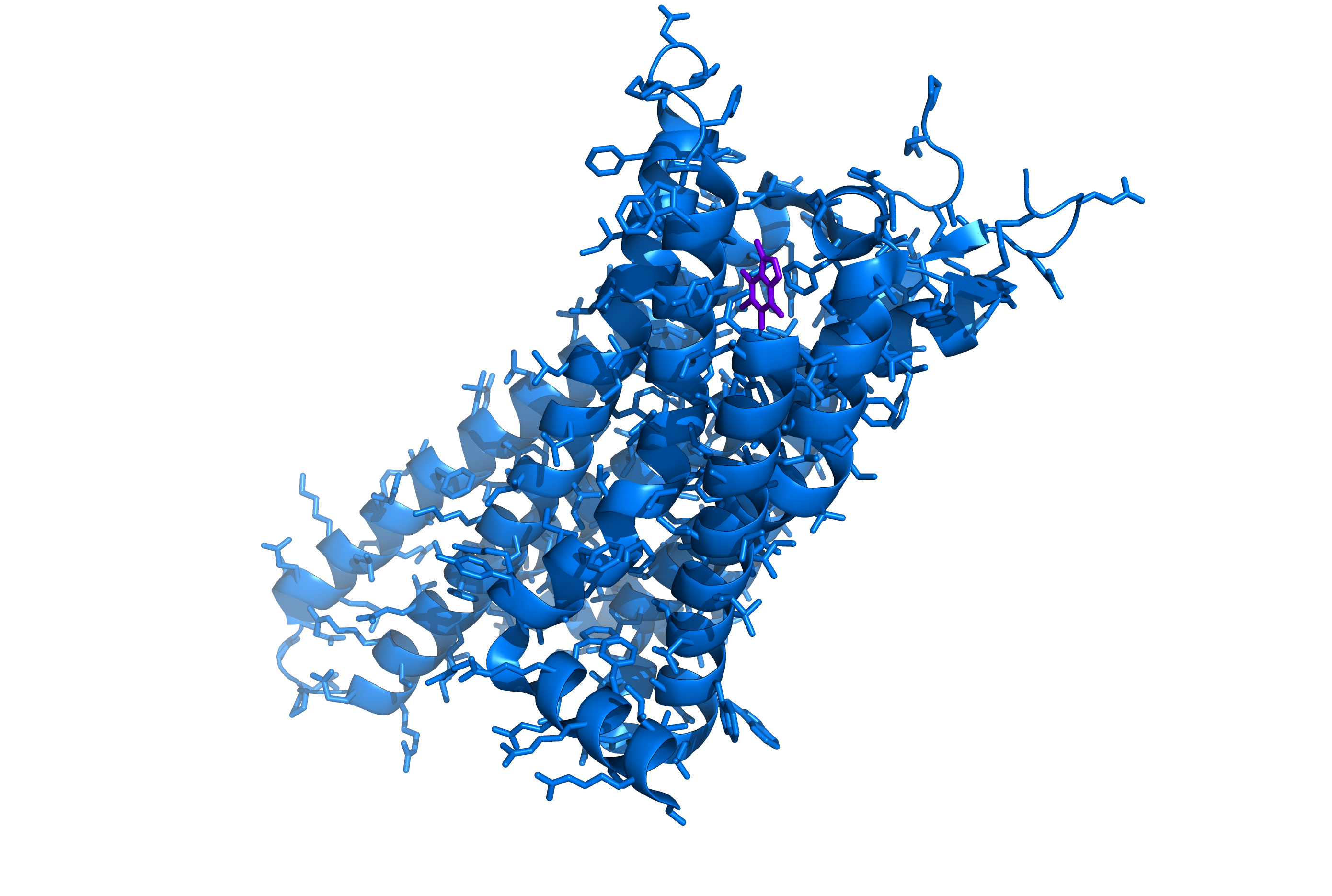
Caffeine (purple) bound to the A2A adenosine receptor (blue).
The protein is an adenosine receptor. Different types of adenosine receptor have different specific activities, but one of the main functions of adenosine receptors is the regulation of drowsiness. When bound to adenosine the receptor interacts with other membrane proteins to, among other things, make you feel sleepy. That’s why we have the purple caffeine molecule inserted into the structure. Caffeine is an adenosine receptor antagonist, it binds the ligand pocket but does not activate the receptor, blocking normal activity and (among other things) making you feel more awake.
In addition to looking like the world’s smallest ninja turtle, caffeine bears a visual resemblance to adenosine. More importantly, the molecular properties are similar enough to allow caffeine to surreptitiously fill in for adenosine.
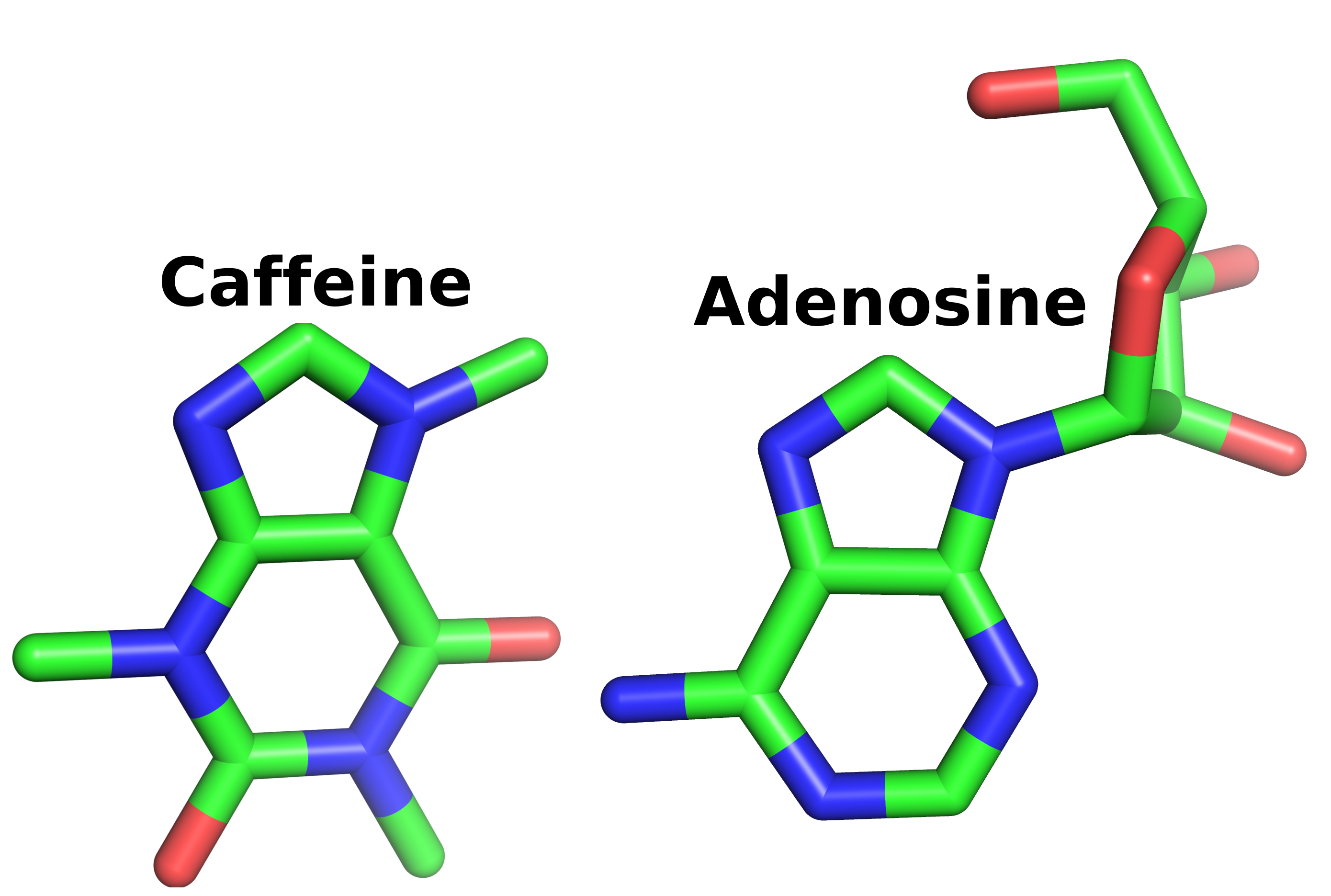
If you don't see the resemblance it may be difficult for us to understand one another.
Normally, adenosine builds up and begins to bind to more and more receptors, which in turn will adopt an active conformation with the most visible change being the shift in the position of the transmembrane helix 6 (H6). Compare the structure of adenosine receptor A2A bound to adenosine below to that of the earlier structure bound to caffeine.
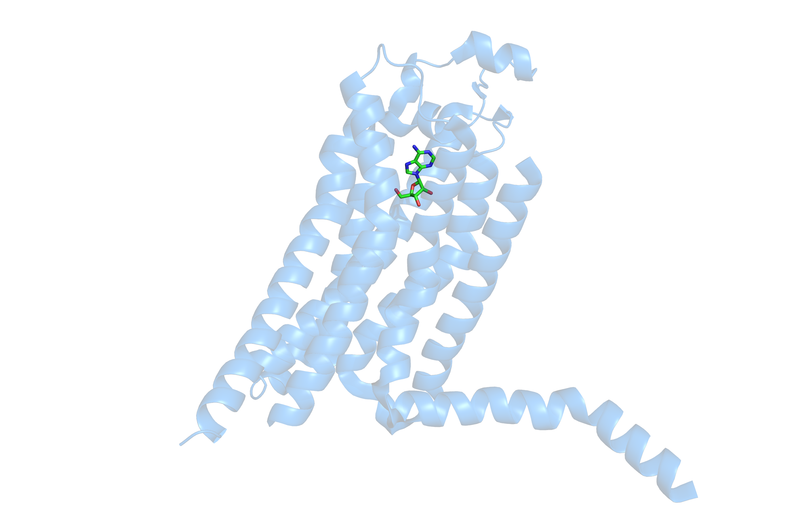
Adenosine bound to the A2A receptor. Notice the change in confomration of an extended alpha helix
As much as humans love caffeine, it’s not the only thing we can put in our bodies to change the way those moist little protein machines go about their business. Many pharmacological interventions for much more serious pathologies work in much the same way: by interacting with proteins and either blocking or altering their normal function.
In the olden days, drugs would largely be discovered by chance: douse a cell culture in a chemical and see what happens. The choice of drug candidate was largely a matter of guesswork (e.g., this molecule Y reminds me of molecule X which does what we want except for deadly side effects, so let’s cross our fingers and try Y). With the readily available computational power we have today, and a whole lot of algorithmic development over the years, drug discovery can be substantially more directed than random screens and hunches. A key technique for determine whether a protein might interact with a given small molecule ligand is molecular docking.
Molecular docking is a computational technique for studying protein-ligand binding interactions. Caffeine is a pretty non-selective binding partner that binds to different types of adenosine receptor more or less indiscriminately, but in fact there are 4 different adenosine receptors in humans and each one has different prevalence and effects in different tissues of the body. Specific antagonists and agonists can hone in on a target effect of a specific receptor while incurring fewer side effects. Thousands of compounds can be screened for binding affinity to a target molecule in a virtual screen featuring molecular docking to determine whether and how well candidate small molecules might bind the target.
Luckily there are several open source tools for molecular docking. The one I used for this experiment is called Smina, itself a fork from Autodock Vina which is itself a successor to Autodock. Other free and/or open source options include rDock, RxDock, and many others.
The Experiment
Smina uses a default scoring function to evaluate the goodness of fit during docking simulations, but you can also provide custom weights for the different terms in the function. A custom weighted scoring function can make a big difference in the outcome of the docking simulation, and this becomes more important the more specialized your application is. The experiment described here aims to optimize the scoring function weighting for re-docking on a small dataset comprised of 11 protein-ligand training pairs and 10 validation pairs. Esben Jannik Bjerrum at Cheminformania published a similar study using particle swarm optimization, and his work was an inspiration for the experiment described here and in fact I based the dataset on the proteins he used in his paper..
We’ll judge the efficacy of the docking simulation and our custom scoring weights based on the root mean square deviation (RMSD) of ligand position from solved structures of each ligand in complex with its binding partner protein. If the docking simulation software was implemented to be differentiable, we could potentially learn optimal weights directly by back-propagating all the way back from the RMSD through the physics simulation to update our weight parameters. Instead, the docking program operates like a black box or oracle, so the individual impact of changing each weight isn’t directly recoverable from the process. This makes the problem a reasonable candidate for a black box optimization or reinforcement learning formulation, and I’ve wrapped the protein-ligand docking process in an RL environment. This converts the docking score (plus any regularization penalties) to a reward which is then passed to a learning algorithm.
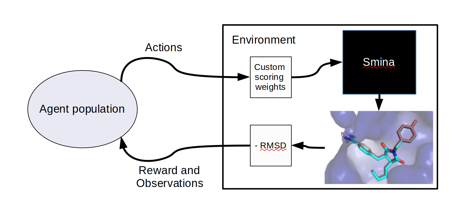
Docking as a reinforcement learning environment.
I chose covariant matrix adaptation evolution strategy as my learning algorithm, evolving the scoring weights directly. It’s also possible to optimize docking indirectly by evolving neural network or other agent policies that in turn generate scoring weights, and in an earlier experiment optimizing for re-docking with a single protein-ligand pair, I found similar results training a neural network as I did evolving the scoring parameters directly. However, without exposing more information to the agent there’s no clear reason to do that, so I didn’t explore neural policies in the larger experiment. Exposing more information in agent observations (and separating observations from the quantity being optimized) is a subject for future work, and there are several other ways to improve protein-ligand docking via machine learning, such as filtering out unpromising ligand candidates with a predictive ResNet-based model.
Covariance matrix adaptation evolution strategy (CMA-ES) is a flexible way to efficiently explore parameter space during evolution. CMA-ES follows the typical pattern of evolution strategies: sampling a population from a distribution, evaluating fitness, and finally updating the distribution based on the population’s top performers. CMA-ES is useful because it increases search breadth when the difference between the best performing and the average agents is large. The difference is stark when compared to an evolution strategy with constant variance, shown here finding a peak on the Himmelblau function:
For a thorough description of CMA-ES (especially applied to reinforcement learning), check out the blog posts from Lillian Weng and David Ha, or if you want to take a wade in the weeds I recommend the tutorial from CMA-ES inventor Nikolaus Hansen.
Results
I ran the experiment 3 times for 20 generations with a population size of 96. After training, the top 4 sets of scoring parameters on the champions leaderboard were evaluated for 50 docking simulations each on both the train and validation sets. That’s about 5X coverage of the (admittedly small) respective data sets, and the reason for docking the same receptor-ligand pairs is because Smina results are sensitive to random seeds and can give somewhat different scores for docking simulations with otherwise identical parameters. I compared the root RMSD based on scoring functions found with CMA-ES to the RMSD obtained using the default scoring function, and from the optimized coefficients reported by Esben Bjerrum. The RMSDs using default or Bjerrum’s scoring functions were also averaged over 50 docking runs on both train and validation sets. Although I never trained on the validation set I did check performance at several points during development, so we can’t call it a test set. Indeed there is more work to be done on this project (including expanding the data sets) and so I’ll need a fresh dataset to test with if I develop DockRL further.
The CMA-ES optimized parameters usually performed a little better than the default scoring function parameters or those reported by Esben Bjerrum. The difference is not enough to propose that CMA-ES should always find a better scoring function (in fact in one training run, the CMA-ES optimized results on the validation set were much worse than than the default scoring function). When comparing to the scoring weights Bjerrum found with particle swarm optimization, remember that Bjerrum was optimizing for a slightly different objective. I used re-docking, but Bjerrum was optimizing for crosss-docking (docking with alternative ligands on the same protein) and therefore found scoring weights that are more flexible. In cross-docking one ligand may induce conformational changes in the protein binding partner that aren’t induced by another, and is thus a slightly different problem.
These are the learning curves for the 3 experimental runs:
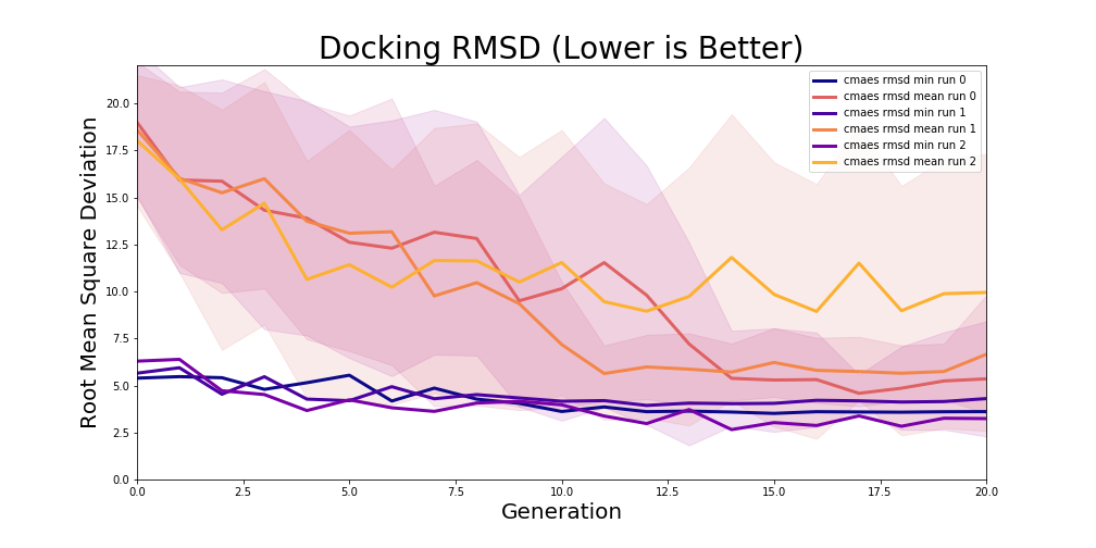
Learning curves for 3 20-generation training runs. Note the large error bounds around the mean population RMSD, which are standard deviation, for CMA-ES.
And the final evaluation results:
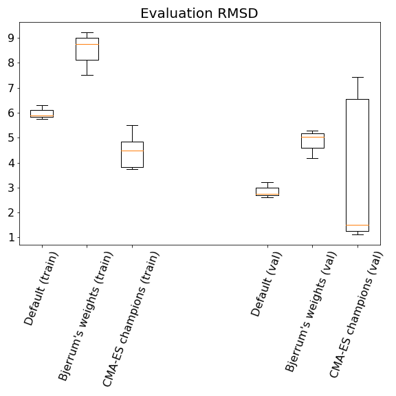
Evaluation after 20 generations.
From 3 experiments I evaluated 12 champions, finding parameters that were not necessarily the same or very similar each time. That’s one advantage of evolutionary strategies: they tend to find a diversity of solutions to a problem. It’s often recommended to use multiple protein structure conformations or even multiple docking programs when conducting a serious protein-ligand docking study, and so using a few different scoring function parameters with similar performance is probably useful as well. That being said, the scoring function parameters found here are not necessarily a good choice for virtual screening for outcomes like binding affinity, as I did not consider outcome metrics other than RMSD in the problem formulation.
The terms of the Smina scoring function are:

gauss(o=0,_w=0.5,_c=8)
gauss(o=3,_w=2,_c=8)
hydrophobic(g=0.5,_b=1.5,_c=8)
non_dir_h_bond(g=-0.7,_b=0,_c=8)
repulsion(o=0,_c=8)
num_tors_div

This experiment used CMA-ES to find the following scoring function weights:

Run 1 scoring parameters:
champion 0 params[-1.27436509 -0.78211046 -1.43731841 -0.62711461  8.08476711 -4.13627455]
champion 1 params[ 0.98503205  1.00482034  0.82207653  1.63228035  5.82537214 -1.87687959]
champion 2 params[-0.50955464 -0.30881923 -0.67250885  0.13769497  7.31995753 -3.37146498]
champion 3 params[-0.97166039 -0.5595893  -1.13461405 -0.32441024  7.78206274 -3.83357019]

Run 2 parameters:
champion 0 params[ 0.86030765 -0.22638877  2.80786698 -1.30804956  2.95815515 -0.9737103 ]
champion 1 params[ 1.52885428 -0.80799741  3.39175208 -1.89033777  3.54156745 -1.55616689]
champion 2 params[ 1.00245422 -0.41628406  3.00158739 -1.49842547  3.1520491  -1.16402611]
champion 3 params[ 0.97804152 -0.30462964  2.88951414 -1.38691413  3.03962265 -1.05280124]

Run 3 parameters:
champion 0 params[ 0.41357491 -0.18255163 -2.61913379 -1.71610385  6.50601953 -2.04936759]
champion 1 params[ 0.76318569 -0.53203977 -2.26980438 -1.36681169  6.15669825 -1.70007063]
champion 2 params[ 0.64379294 -0.41241577 -2.38943701 -1.48640363  6.27636678 -1.81969771]
champion 3 params[ 0.61541451 -0.38431518 -2.41750048 -1.51446684  6.30441191 -1.84774295]

Compare to Bjerrum's cross-docking parameters
(see https://www.cheminformania.com/machine-learning-optimization-of-smina-cross-docking-accuracy/
 and https://linkinghub.elsevier.com/retrieve/pii/S1476927116300214)
Bjerrum params: [-0.0460161, -0.000384274, -0.00812176, -0.431416, 0.366584, 0.0]
This experiment demonstrates an interesting way to pursue docking optimization, albeit with limited data. There’s a lot more that could be added: exposing more information about the protein and ligand in observations, experimenting with other learning algorithms, expanding the dataset, etc.
Thanks for your attention, and if you want to try out DockRL for yourself you’ll find the MIT-licensed Github repository at https://github.com/rivesunder/dockrl. If you do, it’d be great to hear your thoughts and you can connect with me on Twitter @rivesunder.