Synaptolytic Learning: Learning RL Tasks via Pruning Alone
Intro
In early cognitive development human children undergo a period of exuberant synaptogenesis that persists until about 2 years after birth, though the timing of maximal synaptic density differs by brain region (Huttenlocher and Dabholkar 1997). This period of rapid growth is followed by a long period of gradual reduction in synaptic density. Perhaps counterintuitively, the development of complex cognitive functions corresponds to the decrease in synaptic density, rather than during periods of increase (Casey et al. 2015 pdf).
Despite the apparent essential role of synaptic pruning in cognitive development, there is no shortage of gurus and supplement distributors available to take advantage of the questionable assumption that more synapses is equivalent to a better brain. This is probably the result of conflating developmental synaptogenesis with neurodegeneration-related cognitive decline, a different process than developmental pruning altogether that has been cleverly analogized as the difference between sculpting and weathering (Kolb and Gibb 2011). On the other hand, the coincidence of lower synaptic density with the development of higher-order brain functioning also tempts us with an overly simplistic view of synaptic density and cognitive capability. Glial cell proliferation, myelination, and other factors play into neurophysiological dynamics during development and so also must contribute important roles. It seems likely that exuberant synaptogenesis provides a substrate well-disposed to learning at the expense of cognitive capability and metabolic efficiency while pruning results in more effective neural circuitry, but the science is far from settled on these fronts.
The physiological processes behind cognition remains a complex subject with many unanswered questions, but that’s no reason we can’t experiment with a vastly over-simplified view of synaptic pruning as a machine learning paradigm. As artificial neural networks represent a vision of computation loosely based on biological neural circuitry, synaptolytic learning is a way for machines to learn loosely based on the complicated circus of neurophysiological dynamics in the development and maintenance of cognitive capability in biological brains.
Related Work
This work is related to recent work in growing or sculpting sparse networks for machine learning tasks. In particular, this work is related to weight agnostic neural networks, or WANNs, (Gaier and Ha 2019 paper, blog, code). While WANNs are built on top of a neural architecture search strategy called NEAT, with WANNs skipping the inner training loop because all connections share the same weight and do not need to be trained. Unlike WANNs, the learning by pruning is destructive and the size and complexity of the model is therefore bounded by the starting network. Although the weight values are shared (like in WANNs) they are always 1.0. In other words the resulting networks are binary neural networks. Furthermore, WANNs use a diversity of activation functions that not considered in the current implementation of pruning-based learning. Like WANNs, learning by pruning differs from architecture search in general by doing away with a computationally expensive inner training loop used to adjust network parameter values.
A second related nascent body of work is organized around the concept of the “Lottery Ticket Hypothesis” (LTH, Frankle and Carbin 2019). At a high-level of abstraction the LTH states that deep neural networks learn well because they contain one or more sub-networks capable of solving a given task. After training, sub-networks are derived from the full network by removing less relevant portions of the fully trained model (pruning) and re-trained to recover the original performance. Previously, re-training pruned networks has been used as part of an effective compression method allowing models to fit on SRAM for dramatic inference speedups (Han et al.).The recent contribution (and LTH premise) is that these sub-networks can be re-initialized (so long as they are given the same starting values) and re-trained to the same or similar performance as the full-sized network, though sub-network discovery still requires fully training the complete network (Frankle and Carbin 2019).
Prior to its role in LTH, pruning has been used in artificial neural networks since at least the 1980s as a means to improve generalization and inference efficiency (Reed 1993 pdf ). A characteristic shared by these works that distinguishes them from learning by pruning is that regardless of method, pruning is always performed on trained networks. Typically newly-pruned networks are re-trained to recover the performance of the original network. In contrast, the pruning method discussed here is the learning method.
Learning by Pruning
The Environments
I used the PyBullet versions of cartpole balancing and swing-up tasks: InvertedPendulumBulletEnv and InvertedPendulumSwingupBulletEnv. These environments are a implementation of cartpole balancing variants (Barto, Sutton and Anderson 1983). I found that a standard CartPole task is rather easily solved by pruning learners, whether using the Box2D version from OpenAI Gym or another version like the PyBullet environments used here. In the PyBullet balancing environment, capped at 1000 steps, it’s not uncommon to discover a solution in the first few generations, equating to a few hundred thousand steps including every step taken by each policy in every generation over multiple episodes. The reward is +1 for every step and the episode is terminated when the pole falls below a threshold level, making a score of 1000 the best possible return. In training the pruning-based agents, the reported fitness includes a penalty for network complexity which can decrease the return by at most 1.0, so the problem can be considered solved for fitness scores between 999.0 and 1000.0
InvertedPendulumSwingupBulletEnv provides a more difficult task. With the cart/pole system initially in a state with the rod hanging below the cart, an agent must first swing the pole up before keeping the pole balanced as well as possible for the remainder of the episode. This task environment is also capped at 1000 steps and receives a positive reward when the pole is balanced, and negative reward when the pole is below the cart.
Pruning and Selection Method
I compared 2 variants of the learning by pruning scheme. The first variant (mk1) is a genetic algorithm that randomly removes connections in the policy network to form a population of agents that are then tested on the task at hand for multiple episodes. The training procedure retains the elite 1/8 of the population from the last generation, the all-time best 1/8, and the all-time best single policy, and these policies are inherited as the starting point for the next generation, which is then mutated stochastically where the only mutation availabe is the removal of connections. The mutation rate is adaptive, but I did not investigate in-depth whether the adaptation mechanism provided any benefit over a set rate. At every generation, the probability of removing any given connection is determined as the standard deviation mean square difference between the average number of connections in the general population of policy networks and the average number of connections in the elite population:
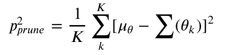
Where  is the mean number of connections in the general population,
  are the parameters for each elite policy
  , and
, and  is the total number of elite agents. The mutation rate is clipped etween 0.1% and 12.5%.
Genetic algorithms often incorporate recombination, where parameters from two or more parents may be swapped to produce variable offspring before mutations are applied. In this iteration of the pruning methods described here no recombination was applied, in part because of the extremely simple single-hidden layer architecture of the networks investigated in this experiment. Another reason I wanted to avoid using recombination was to experiment with purely destructive learning algorithms: a deleterious synaptic loss cannot be recovered for a given agent and it’s offspring, although it may be supplanted by the fitter progeny of competing policies retaining the lost connection. I deviate from the purely destructive learning algorith in the second version of the pruning-based learning algorithm.
The second variant of pruning-only learning (mk2) has more in common with distribution-based evolutionary strategies. Instead of inheriting network policies from parent generations that are than pruned, each generation is intialized anew with the probability of pruning any given connection given by the frequency of that connection in the elite section of the preceding population. These probabilities are clipped at 5% and 95%, so no matter how rare or common a connection is in the elite population it still has at least a 5% chance of being pruned or retained by every member of the next generation. Additionally, a few (half the elite population in these experiments) of the best policies are carried over intact to provide some training stability.
Covariant Matrix Adaptation Evolution Strategy
I implemented a naive covariance matrix adaptation evolution strategy (CMA-ES or CMA for short) as a point of comparison for the pruning-based methods. The current implementation used for this experiment is based on the description at A Visual Guide to Evolution Strategies, however any bugs/mistakes in the implementation are my own doing. Actually I have already identified one deviation from canonical CMA-ES. In my implementation I calculate covariance matrices for each layer-to-layer weight matrix separately. In a proper CMA-ES implementation a single covariance matrix should be computed for all parameters. The current implementation works pretty well and qualitatively behaves as expected, exhibiting reasonable exploration and fine-tuning during training, but it is possible that fixing this mistake (issue) will make the pruning-based algorithms less competitive next to CMA-ES.
A covariance matrix is used to define a distribution from which parameters are sampled at each generation. The mean and covariance for each weight is computed as follows:
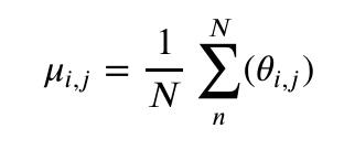
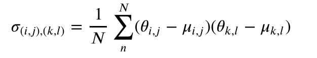
Where  is the mean value for a given weight,
  is the weight value, and
  is the covariance. Subscripts define the connections, for example between nodes i and j and as implied by these subscripts, computing the covariance matrix involves one and two loops wrapping the mean and covariance equations above, respectively.
Shared Characteristics of all Policies
All policies have a single hidden layer with 32 nodes and use tanh activation. The observation space is a length 5 vector and the action is a single continuous number between -1 and +1. Training continues for at least 100 generations until a solution threshold is reached (a return of 999.5 on the balancing task or 880.0 on the swingup task). The balancing task utilizes a static population of 128 at teach generation while the swingup task doubles that number for a population of 256. Policy runs are repeated 8 times for each member of the population at each generation.
Results
Example episode demonstrating the performance of the mk2 pruning algorithm champion network.
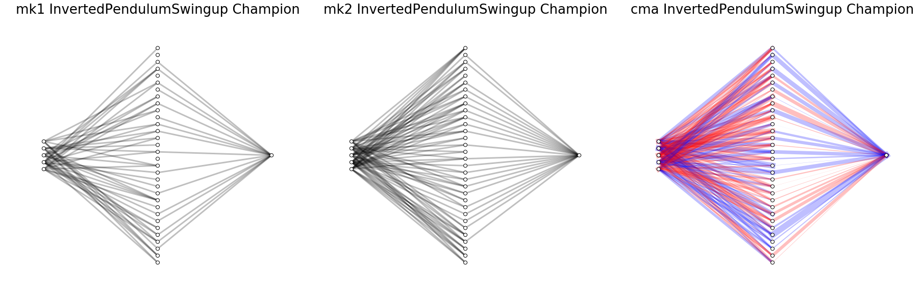
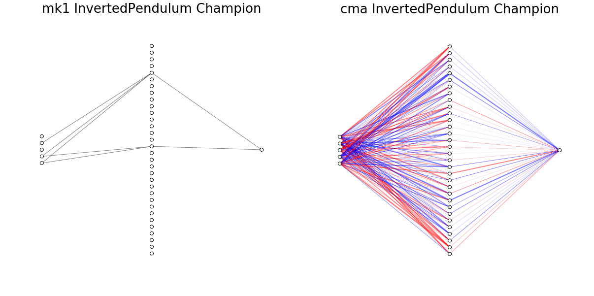
Champion networks learned by each training method. The red and blue coloration of connections in the CMA network represent negative and positive weights, respectively, while the thickness indicates the absolute magnitude of each connection. The connections in the mk1 and mk2 networks are always 1.0.
Both mk1 and mk2 pruning methods are able to solve the InvertedPendulum and InvertedPendulumSwingup tasks. In terms of wall time the solutions are found pretty quickly. Total steps required by the mk1/mk2 methods to pass a solution threshold solution are comparable to CMA-ES, although mk2 is a bit worse than the other methods.
In this initial experiment I focused on finding solutions to each task, truncating training after meeting a solution threshold for each task after at least 100 generations. Consequently the champion networks do not represent minimum description length (MDL) solutions. This is visually apparent in the mk2 champion network for InvertedPendulum and less blatant but still obvious in the mk2 champion network for InvertedPendulumSwingup, where we can see that many of the connections from observations to inputs don’t affect the final outcome.
The mk1 algorithm tends to do a better job of simplifying connections, finding a solution to the balancing task with only 7 connections. Without individually optimizing hyperparameters for each algorithm it’s not clear if the mk1 method is intrinsically better at finding a more efficient policy, if the mk2 method intrinsically has trouble overcoming local optima to find more efficient policies, or if they’ll both find similarly simple solutions eventually.
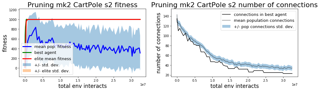
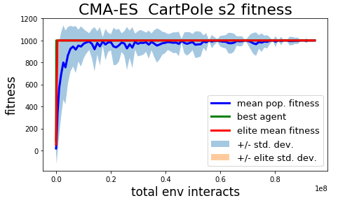
All 3 methods solve the balancing task pretty quickly.
| Method | Steps to solve (R > 999.0) | Best agent final performance |
|---|---|---|
| CMA | 1.928e+05 +/- 1.3762e+05 | 1.000e+03 +/- 0.000 |
| Pruning mk1 | 2.507e+05 +/- 9.224e+04 | 1.000e+03 +/- 0.000 |
| Pruning mk2 | 2.743e+05 +/-9.097e+04 | 1.000e+03 +/- 0.000 |
Table 1: Learning performance on `InvertedPendulum` pole-balancing task. As evident in the "Best agent final performance" column, this task is too easy to be interesting in this context. Of the methods tested the mk1 algorithm found the simplest network that solves the problem.
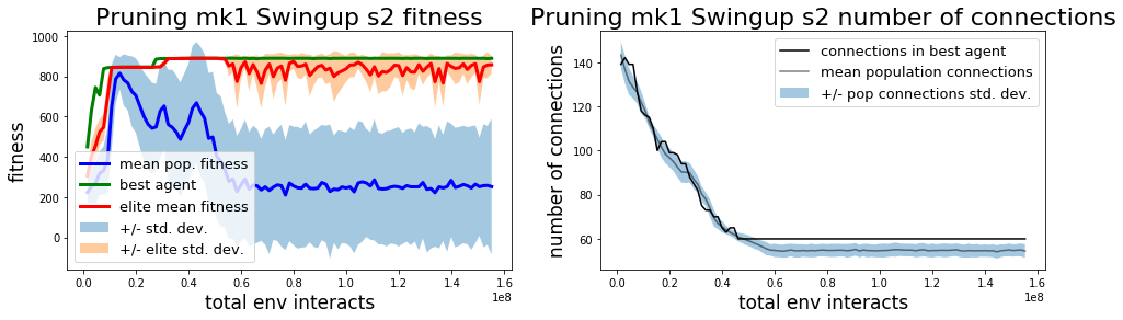
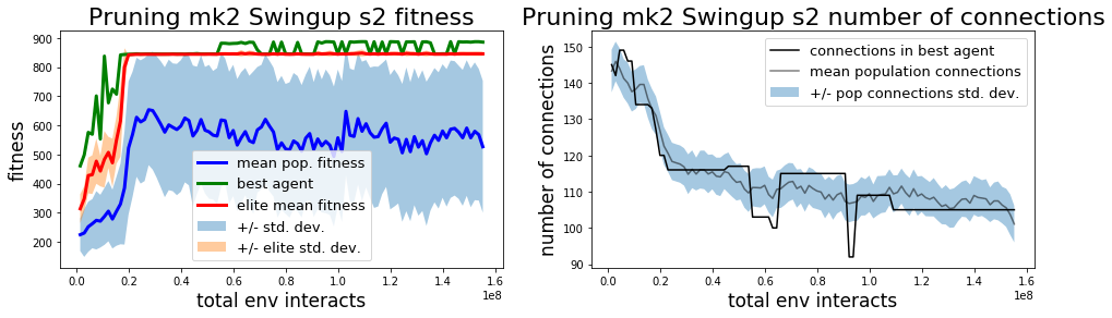
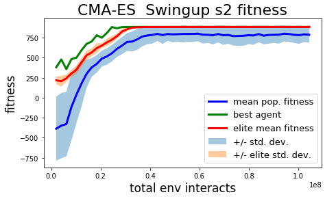
| Method | Total steps to solve | Best agent final performance |
|---|---|---|
| CMA | 3.823e+07 +/- 1.931e+07 | 8.679e+02 +/- 4.244e+01 |
| Pruning mk1 | 3.4301e+07 +/- 6.432e+06 | 8.895e+02 +/- 3.5502e-01 |
| Pruning mk2 | 6.656e+07 +/- 1.095e+07 | 7.767e+02 +/- 2.479e+02 |
Table 2: Learning performance on `InvertedPendulumSwingup` task. "Best agent final performance" statistics are associated with a run of 100 episodes using the champion policy from each method.
The mk1 pruning algorithm performed the best out of the 3 algorithms tested on the more difficult InvertedPendulumSwingup task, but with only 3 seeds tested so far luck may have played on outsized role in the results. Results in final performance may also vary with prolonged training, as in the current experiment training is truncated after passing a return threshold and training for at least 100 generations. The difference in sample efficiency between the mk1 pruning algorithm and CMA is probably not significant (mk2 is probably a little slower), but the final performance of the best agent found with mk1 does seem to be better.
It doesn’t make too much sense to compare the complexity of networks found by pruning and found by CMA. Networks found with CMA (albeit with no regularization) maintain all connections and each connection is real-valued, unlike the pruning networks which can either have a connection or not, represented by weights of 1.0 or 0.0, respectively. The mk1 pruning algorithm tends to find simpler networks while the mk2 algorithm has a greater number of futile connections leading nowhere at generation 100 when training is stopped. The mk2 algorithm also seems to represent a greater variety in terms of the policy strategies (see below) and the variation in total number of connections in the population at each generation. Allowing training to continue may eliminate some of the differences in the policy networks found by mk1 and mk2 methods (or not). The difference in performance and apparent difference in exploration preferences between mk1 and mk2 algorithms could be down to mk2 being a more random policy (like comparing two DQN variants with different epsilon values) and this difference might disappear with individual optimization of each algorithm.
Exploitation vs Exploration
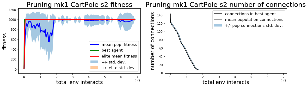
By observation, the mk2 method seems to be more prone to explore than mk1. This is starkly demonstrated in the gif below demonstraing examples from the top 4 elite policies at generation 100 for each method. It’s also apparent in the popultion connection statistics in the learning curves. Of course, this may be an artifact of the hyperparameter settings and could disappear when each method is optimized individually.
A plausible explanation for the tendency of the mk2 method to explore more is the choice of maximum and minimum values of the pruning probability matrices in the mk2 method, set at 95% and 5%, respectively. This means that even if every member of the elite population shares a connection (or lack of connection) between a given pair of nodes, there is still a 5% chance that any given individual in the next generation will differ.
mk1 and mk2 elites attempting the swing-up task.
What’s Next?
More seeds and more interesting environments. The cartpole style InvertedPendulum tasks investigated here, even the swing-up variant, are decidedly on the “too-easy” side of the Goldilocks scale for interesting RL problems.
Investigating biologically plausiblee pruning algorithms, and longer training sessions. Some recent work on artificial neural networks including a Hebbian component for meta-learning may provide inspiration (e.g., Miconi et al. 2018a, Miconi et al. 2018b, and Miconi 2017).
Although the current experiment was successful in determining the ability of pruning-only algorithms to learn simple tasks, we didn’t investigate the more interesting challenge of finding minimal policy networks. Is pruning a good method for finding MDL solutions to reinforcement learning? How does pruning compare to growth-based algorithms like NEAT and WANN in this regard? The latter question is interesting in light of the apparent reliance of mammalian cognitive development on pruning for learning. If there’s no advantage to destructive learning, why do humans make so many extra synaptic connections only to remove them later? An interesting potential explanation is that a big population of possibly redundant neural circuits is more capable of learning new things (via pruning) than highly optimized MDL circuitry. This would suggest that ideal (machine) learners may benefit from alternating periods of exuberant synaptogenesis and selective synaptolysis, perhaps with learned triggers for when to pursue either strategy.
This project has a github repo
Bloopers
Failure can be more interesting than success, and more informative to boot.
Policy found by mk2 method by the 4th agent in the elite population at generation 100.
The policy in the gif above doesn't quite get the bump and balance move right the first time and starts swinging the pole erratically and running into the hard stops set in the environment xml file. My interpretation of this failure mode is that it may be useful to modify the environment to give the agent more room to work with.